Market Basket Analysis (MBA) is a data mining technique and rule-based algorithm that can learn through relationships. MBA can be greatly utilized within ecommerce and marketing strategies which can allow for enhancing more productive decisions that will benefit not only consumer sales but improve the ease of the shopper experience.

When we walk down a grocery store aisle, we expect to see certain items placed together that helps us shop quickly and find the items that we want easily. For example, the cereal aisle will also have otameal, tea, coffee, coffee filters, and sugar. While as humans, we might be able to make an intuiation and basic observation that coffee and tea should be placed near each other, with Market Basket Analysis we are able to optimize our decisions for where to place the many items in a groacery store.

Market Basket Analysis also provides insight into how stores should market their items and target customers. If a customer purchases item A, and we know that item B is frequently purchased with item A, then we might consider targeting item A to that customer. With MBA we can determine how to consider more advantageous group discounts, and even go one step further in developing a recommmendor system for ecommerce shoppers.

MBA is considered a type of rule-based learning. A rule might look like: IF a customer bought tortilla chips, THEN they will also buy salsa.

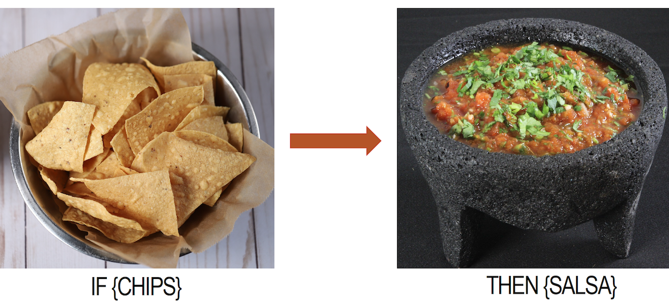
Mining retail datasets like this is done to find a number of relations:

• Complementary products: products which are often bought together, like chips and salsa
• Substitute products: products which replace each other, like Coke and Pepsi
• Trigger products: products which when bought trigger other purchases
• Common Baskets: combinations of products that are often bought together

Setting up Market Basket Analysis

Let’s now review the theory behind Market Basket Analysis and the steps needed to process a dataset.

Step 1: A list of transactions

In order to run the market basket analysis, we must first start with a list of transactions:

Transaction 1: 'Apple', 'Beer', 'Rice', 'Chicken'
Transaction 2: 'Apple', 'Beer', 'Rice' 
Transaction 3: 'Apple', 'Beer'
Transaction 4: 'Apple', 'Bananas'
Transaction 5: 'Milk', 'Beer', 'Rice', 'Chicken'
Transaction 6: 'Milk', 'Beer', 'Rice'
Transaction 7: 'Milk', 'Beer'
Transaction 8: 'Apple', 'Bananas'

basket = [['Apple', 'Beer', 'Rice', 'Chicken'], 
       ['Apple', 'Beer', 'Rice'], 
       ['Apple', 'Beer'], 
       ['Apple', 'Bananas'], 
       ['Milk', 'Beer', 'Rice', 'Chicken'], 
       ['Milk', 'Beer', 'Rice'], 
       ['Milk', 'Beer'], 
       ['Apple', 'Bananas']]

Step 2: Transaction Encoder

Next use TransactionEncoder to transform the list of transactional items into dummy variables which is suitable for computating text data such as in Machine Learning and Statistical Analysis methods.

# Instantiate
te = TransactionEncoder()

# Fit and Transform the data into True and False (1 and 0)
item = te.fit(basket).transform(basket)

# Create DataFrame
df = pd.DataFrame(item, columns = te.columns_)

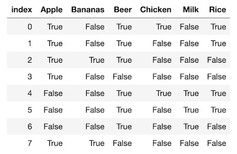
With the dataset transformed into True and False, we can begin to utilize the data by making observations through data visualizations and some quick calculations. Exploring the data before applying a rule base learning algorithm such as Apriori Algorithm can be helpful for making some first order observations.

Below is a table of the sum of each item purchased for all transactions individually and when purchased with another item. We can see that Apples, Beer, and Rice are the top most frequent purcahses. I have as well plotted a contingency heatmap which is a nice visual aid for viewing the frequency co-purcahses.

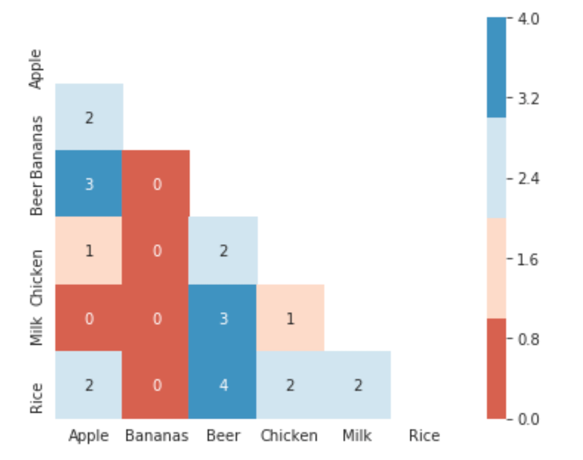
We can see from the contingency heatmap that Beer & Rice were co-purchased together 4 out of the 8 transactions and Beer & Milk and Apple & Beer were purchased 3 out of the 8 transactions. While here in this example, the heatmap is a nice visual aid, for Big Datasets that contain thousands of items, a contingency heatmap will not be able to be helpful. As well, if a customer purchases beer, what is the likelihood that the customer will also purchase a bag of rice? Or what is the likelihood that if the same customer purchases rice will be beer? Is this likelihood the same for both cases? Just because within this dataset, we see that there is a co-purchase between rice and beer, should a company invest time in money in marketing campaigns and consumer strategy that will focus on the purchase of beer and rice?

In order to answer these questions, as data scientists we can apply an Apriori Algorithm which will determine the likelihood of co-purchases.

Step 3: Apriori Algorithm

Apriori Algorithm is an association rule algorithm. Association rules “help uncover all such relationships between items from huge databases”. The Aipori Algorithm groups the list of items into antecedents and consequents. The antecedent is what the customer purchased while the consequent is the purchase result. For example, if a user purchases beer (antecedent) then they will purchase rice (consequent). We can see from the sample dataset above that if a customer buys beer (antecedent) then the customer buys rice (Consequent) for 50% of transactions (4 transactions/ 8 total transactions). We can see here that the antecedent and consequent are setup as an if (antecedent) then (consequent) statement.

Apriori Algorithm quantifies the likelihood of a customer who purchases item A who will also purchase item B.

Apriori Algorithm provides four components: Support, Confidence, Conviction, and Lift:

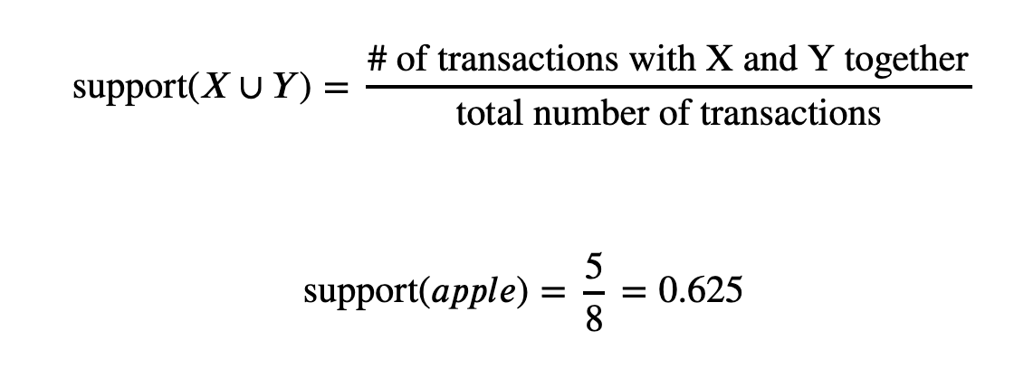
We can then set a support threshold where the support value means the item has a meaningful outcome on sales. Therefore, identifying all items within all transactions where items contain a support threshold equal or greater than the set value. Confidence signifies the likelihood of item Y being purchased with item X. This is also known as conditional probability P(Y|X). The conditional probability of P(Y|X) is the probability of itemset 𝑌 in all transactions given the transaction already contains 𝑋. The drawback of confidence is that it only takes into account the popularity of X, and not the popularity of Y.

Lift takes into account for popularity of Y which thus accommodates for the drawback present in calculating confidence. More precisely lift signifies the likelihood of item Y being purchased when item X is purchased, while taking into account the popularity of Y. If Lift > 1, then Y is likely bought with item X. Lift < 1, then Y is unlikely bought with item X.

The lift of purchasing beer and rice together is 1.3 which means that the likelihood of a customer buying both beer and rice together is 1.3 times more than the chance of purchasing beer alone.

Leverage is the difference in support of the larger group, than would be expected if the antecedent and consequent were independent:

Conviction is the measure of the dependence of the consequent on the antecedent: A high value denotes that we always purchase the C with the A.

APRIORI ALGORITHM EXAMPLE

Creates a DataFrame with 2 columns with Support value and Itemset, where:

• min_support = frequency of occurance in the dataset
• max_len = upper length

 frequent_itemsets = apriori(df, min_support=0.1, use_colnames=True, max_len = 4)

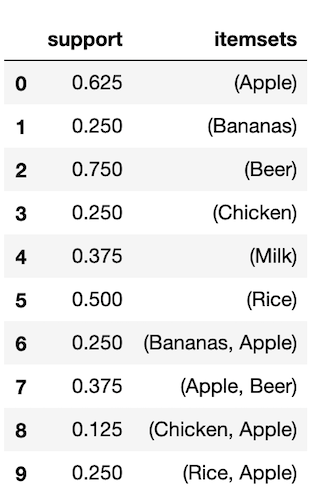
Create a DataFrame with a list of antecedents, consequents, antecedent support, consequent support, support, confidence, lift, leverage, conviction

association_rules = association_rules(frequent_itemsets, metric="lift", min_threshold=1)

Step 4:

Now we can create a recommender system based off of the lift value. For example, if a consumer purchases Milk (antecedent) provide all consequents where the lift value is equal or greater than 5 which means the customer is at least 5 times more likely to purchase item B (consequents) when purchasing item A (antecedent). Another method is to sort the lift values where the output lists the top 3 consequents with the greatest lift values.

For more details, please visit my github!

Links for Reference

https://towardsdatascience.com/mba-for-breakfast-4c18164ef82b https://www.youtube.com/watch?v=WGlMlS_Yydk&t=8s https://towardsdatascience.com/association-rules-2-aa9a77241654 https://towardsdatascience.com/complete-guide-to-association-rules-2-2-c92072b56c84